“By far, the greatest danger of Artificial Intelligence is that people conclude too early that they understand it.”

–Eliezer Yudkowsky

Reinforcement Learning is one of the prominent forefronts of artificial intelligence, though it is much further from the spotlight as compared to the Neural Networks and Support Vector Machines that are finding many business and practical applications. Through this series, I hope to alleviate this lack of knowledge and provide you with an introduction into the world of RL.

Most of this blog stems from the textbook Reinforcement Learning by Richard Sutton and Andrew Barto but takes a more practical approach with less focus on the theoretical details.

As for difficulty, this will be focused towards people who have never touched RL or even machine learning before. I will be going over mathematical equations and python code but those can be ignored if you aren’t interested in the technical details.

Code used:

• Python file
• Jupyter Notebook

Why Reinforcement Learning?

So why use Reinforcement Learning when there are all sorts of Neural Networks, decision trees, and SVMs exist?

1. Data: RL does not assume data is sampled from an independent and identically distribution (i.i.d.) like in other forms of machine learning. In real life, data is usually highly correlated, e.g. an action chosen in a video game might have an impact several time steps later. Additionally, RL has no need for labeled data which can be costly and time consuming to obtain.

2. Adaptiveness: RL is able to adapt quickly to new unseen situations and performs well in highly complex states without requiring prior knowledge to provide useful insights.

3. Intelligence: RL has the potential to attain superhuman capabilities. Supervised machine learning generally uses data collected from humans and emulates that behaviour. Whereas reinforcement learning performs the tasks itself and can, in some cases, outperform the top humans. Because of this, some see RL as the most likely path to achieving Artificial General Intelligence (a machine as capable as a human in every aspect).

$k$-armed Bandits

No this is not about mutant highway robbers, this about slot machines and choices. Consider a slot machine (often referred to as a 1-armed Bandit), but in this case, it has $k$ levers to pull, each leading to a play on the machine with different, independent odds of winning. In order to maximize one’s winnings over repeated plays, one would seek out the highest performing levers and keep pulling them.

Here’s the setup for this environment in python:

import numpy as np

q = np.random.normal(0.0, 2.0, size=10)
std = 0.5

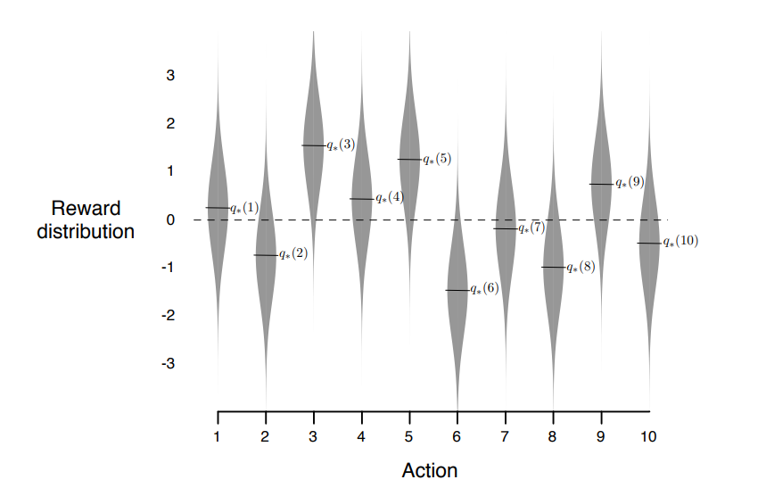
We call the choice we make of the $k$ levers as the action at time $t$, denoted as $A_t$, and the following reward as $R_{t+1}$ (the time is different since technically the reward occurs in the next time step but you’ll see it expressed both ways in literature). We define the quality of taking action $a$ as the expected reward resulting from it:

Where the $*$ represents the optimal (true) of action value function, generally we don’t have access to this so we have an estimate denoted as $q(a)$.

At any time step, there must be an action with the highest estimated value. Always choosing this action is known as exploiting, and to choose any non-maximal action is exploring. The trade-off between these 2 options is short term gain in exploitation, or long term gain in exploration as it allows us to eventually find the real highest value if our estimation is wrong.

Action Value Estimation

So how do we update the action value function $q(a)$ so that it better approximates $q_*(a)$? One idea is to keep an average of the returns that occurred from taking that action. We can do this in constant time and space is to keep track of a count variable and update using:

Here’s the accompanying code:

q_a = np.array([0.0] * len(q))
n_a = np.array([0] * len(q))

for _ in range(5000):
    action = np.random.randint(10)
    reward = np.random.normal(q[action], std)
    n_a[action] += 1
    q_a[action] += (reward - q_a[action]) / n_a[action]

$\epsilon$-greedy Methods

Given our action value function, how do we decide which action to take? If we only choose the greedy (highest estimated value) action, the agent might spend all its time exploiting a good action without ever exploring the optimal action.

We can combat this by using $\epsilon$-greedy methods, where we have an $\epsilon$ chance to take an action at random (includes the greedy action) and select the greedy choice otherwise. However, if we have a constant $\epsilon$, then even after an infinite number of iterations and convergence to the optimal value function, we will not take the optimal (which is now the greedy option) action with more than $(1-\epsilon) + (1/n)\epsilon$ chance, where $n$ is the total number of actions possible.

q_a = np.array([0.0] * len(q))
n_a = np.array([0] * len(q))

def greedy_epsilon(epsilon):
  for _ in range(5000):
    action = None
    if np.random.random() < 1 - epsilon:
      action = np.argmax(q_a)
    else:
      action = np.random.randint(10)
    reward = np.random.normal(q[action], std)
    n_a[action] += 1
    q_a[action] += (reward - q_a[action]) / n_a[action]

greedy_epsilon(epsilon = 0.1)

Optimistic Initialization

One way to improve this with a bit of knowledge about the rewards is to initialize the values of $q(a)$ optimistically, as in, we over estimate all of the expected rewards so that each reward is explored at least once early on in the algorithm (since every initial value is eventually the greedy choice since they are higher than those of any true ones). In our example, we would just change the first line to:

q_a = np.array([5.0] * len(q))

Moving Rewards

Consider a situation where the rewards of the levers slowly change over the course of time. In this case, it would make sense to weigh recent rewards more compared to past rewards. We can weigh our update using a step-size $\alpha \in (0, 1]$ instead:

We can also set $\alpha$ to be a function that changes over time (e.g. setting it to $\frac{1}{n}$ makes it the sample average from above).

def alpha(action):
  return 1 / n_a[action]
  # return 0.1

Softmax Action Selection

In $\epsilon$-greedy methods, we do exploration randomly, with no discernment of which non-greedy action should be tried. In Softmax Action Selection, we take into account how close the estimates are to being maximal by sampling from the possible actions, each with probability:

Where $\beta$ is an adjustable parameter that controls the degree of exploitation (if $\beta = \infty$ it becomes greedy action selection). Here’s an implementation of it:

q_a = np.array([0.0] * len(q))
n_a = np.array([0] * len(q))

def softmax(x):
    return np.exp(x) / np.sum(np.exp(x), axis=0)

def softmax_action(beta):
  for t in range(5000):
    action = np.random.choice(
        np.arange(len(q_a)), 
        p = softmax(q_a)
    )
    reward = np.random.normal(q[action], std)
    n_a[action] += 1
    q_a[action] += alpha(action) * (reward - q_a[action])

softmax_action(beta = 1)

We can also make $\beta$ a changing function over time for better convergence performance (usually exponentially increased so it approaches greedy).

Upper-Confidence Bound Action Selection

In Upper-Confidence Bound (UCB) action selection we take into account how close the estimates are to being maximal and also the uncertainty of estimates using:

Where $a$ is the action, $t$ is the current time step, $n_a(a)$ is how many times $a$ was selected, and $c$ is an adjustable parameter that controls the degree of exploration. So the $q(a)$ term measures the how maximal the estimate is, the $c\sqrt{\frac{ln(t)}{n_a(a)}}$ term measures how uncertain the estimate is. Here’s an implementation of it:

def ucb(c):
  for t in range(5000):
    action = np.argmax([q_a[i] + c * np.sqrt(np.log(t+1)/np.max([n_a[i], 1])) for i in range(len(q_a))])
    reward = np.random.normal(q[action], std)
    n_a[action] += 1
    q_a[action] += alpha(action) * (reward - q_a[action])

ucb(c = 2)

This is better than softmax since it also takes into consideration the number of times an action has been tried, e.g. if the optimal action is estimated as the least expected reward at the start, UCB is guaranteed find it where Softmax could by chance, never explore it.