In the previous part we outlined the basics of the value function and how to choose actions given it. Today, we will formally define a general representation of an environment and generate a policy from it.

For the previous parts:

Part 1: Reinforcement Learning

Code used:

• Python file
• Jupyter Notebook

Markov Decision Processes

A Markov Decision Process (MDP) is a sequence of decision making events where the outcome is determined partly randomly and partly based on our action. They satisfy the Markov property: all conditional probabilities of future states depend only on the current state and not past ones. MDP leads to a sequence of States ($S$), Actions ($A$), and Rewards ($R$):

Given State $s$ and Action $a$, we define probabilities of Next State $s’$ and Reward $r$ with $p(s’,r|s,a)$. The representations of these states and actions vary wildly and have a strong impact on the performance of the agent.

The randomness comes from stochastic environments, where the split between environment and agent is generally defined as the limit of absolute control. Even things like motors and muscles are sometimes considered part of the environment as they can exhibit random unexpected behaviour.

Goals and Rewards

We need to define and measure our goal in order for the agent to know how well its performing. This involves creating an associated reward function that defines what we want the agent to accomplish, but not how we want it to achieve it. For example, if we want an agent to move to a certain location, we can use the negated distance from goal as the reward (further is worse so more negative).

Generally, we define the reward function as the expected return for future rewards, denoted $G_t$. Since the task might never end, we discount future rewards with rate $\gamma$ between 0 and 1:

Although this is an infinite sum, as long as the discount is less than 1 and reward stays constant, the return stays finite as well.

In order to combine the episodic and never-ending scenarios, we assume a constant state of reward 0 after the terminal step in episodic cases so it too is infinite without any effect to the reward function.

The design of this function is paramount to the agent’s performance. Suppose we were to simulate an agent in a room where it needs to reach the door, where it receives a reward of +1, and at every time step it suffers a reward of -1. And say the simulation terminates whenever a wall, window or door is reached. In this situation, the agent would quickly learn that throwing itself on a wall or out a window is the most optimal solution, as it incurs the least negative reward.

Value Functions

After we decide our policy $\pi (a|s)$ (probability the agent takes action $a$ in state $s$, can be deterministic or stochastic depending on action selection) with methods from last post, we can define how rewarding it is for an agent to be in a certain state.

One way to achieve this is to create a state value function $v_\pi(s)$, which defines the value being at state $s$ and following $\pi$ from then on:

Another way is a state-action value function $q_\pi(s, a)$, which defines the value of taking action $a$ in state $s$ and following $\pi$ from then on:

Relational Equations:

Value functions satisfy a recursive relationship:

This is known as the Bellman Equation, essentially a weighted average of all possible actions, next states, and discounted future rewards.

Optimization Policies

To improve our policies performance, we attempt to reach a policy greater than or equal to all others, the optimal policy $\pi_*$. We can do this by first trying to reach an optimal value function:

Given an optimal value function, any policy that assigns nonzero probabilities only to maximal actions are optimal policies.

Although it is possible to solve these equations directly, we require knowledge of the dynamics of the environment, the Markov property, and enough computing power as the number of states and actions could be arbitrarily large. If we solve these, then we can directly compute $\pi_*$:

But generally we do not know the dynamics of the environment nor do we have the capability to compute the direct solution. Thus, we need to find a way to reach approximate states of these optimal value functions.

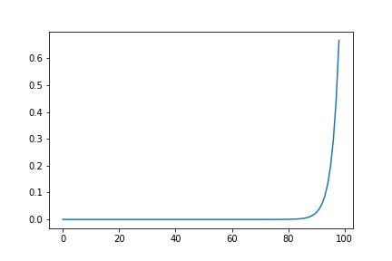
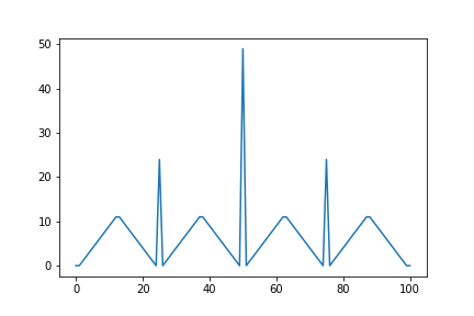
A Gambler’s Game

Before approximating the value functions, let’s consider a game: a gambler starts with some amount of money, their goal is to bet on weighted coin flips, winning back double his bet for each head, and losing his bet for tails. He wins when he has 100 dollars and loses upon reaching 0 dollars. Here is the python code for this:

import numpy as np

# States represent how much money our gambler has, with range [0, 100] inclusive
V_s = np.zeros(101)
NUM_STATES, NUM_ACTIONS = 101, 50

# Reward of +1 at 100 and 0 otherwise
def reward(state):
  return int(state == 100)

# Gambler can bet at most up to his money, or the amount of money that gets him to 100 if heads
def get_actions(state):
  return list(range(0, min(state, 100 - state)))

def get_states():
  return list(range(1, 100))

# Probability of Heads
p_h = 0.4

# Calculate probability and new state, reward transitions
# There are 50 actions to take (actions in [1,50] inclusive)
# Returns list of (next_state, reward, probability)
def transitions(state, action):
  return [
    (state + action + 1, reward(state + action + 1), p_h),
    (state - action - 1, reward(state - action - 1), 1 - p_h),
  ]

# Set up training parameters
DELTA_LIM = 0.0000000001
DISCOUNT = 1

Policy Evaluation

Now, to approximate optimal value functions, we can use Iterative Policy Evaluation. Which calculates state values using dynamic programming until the recursive formula becomes stable with less than $\Delta$ change between iterations. Let $v_k, v_{k+1}$ represent the current and next approximate value functions we have for the optimal $v_*$.

Here’s the accompanying code:

def policy_evaluation(V_s, policy):
  delta = DELTA_LIM + 1
  
  while delta > DELTA_LIM:
    delta = 0
    for state in get_states():
      old_state = V_s[state]
      
      expected_reward = 0
      for action in get_actions(state):
        action_reward = 0
        for next_state, reward, prob in transitions(state, action):
          action_reward += prob * (reward + DISCOUNT * V_s[next_state])
        expected_reward += action_reward * policy[state, action]

      V_s[state] = expected_reward
      delta = max(delta, abs(old_state - V_s[state]))
    
  return V_s

Policy Improvement

Iterative Policy Improvement compares the values of taking each action at each state, and if they’re better than their respective state values, then the policy is changed accordingly.

Here’s the accompanying code:

def policy_improvement(V_s, policy):
  stable = True

  for state in get_states():
    old_action = np.argmax(policy[state])
    rewards = np.zeros(NUM_ACTIONS)

    for action in get_actions(state):
      for next_state, reward, prob in transitions(state, action):
        rewards[action] += prob * (reward + DISCOUNT * V_s[next_state])

    policy[state] = np.eye(NUM_ACTIONS)[np.argmax(rewards)]  
    stable &= (old_action == np.argmax(policy[state]))
  
  return policy, stable

Policy Iteration

To combine Policy Evaluation and Policy Improvement, we use Policy Iteration, which simply runs one cycle of Policy Evaluation then one cycle of Policy Improvement over and over, similar to Expectation Maximization in other contexts.

Here’s the accompanying code:

def policy_iteration():
  V_s = np.random.random(NUM_STATES)
  V_s[-1] = 0

  policy = np.zeros((NUM_STATES, NUM_ACTIONS))
  policy[:, 0] = 1

  stable = False
  while not stable:
    V_s = policy_evaluation(V_s, policy)
    policy, stable = policy_improvement(V_s, policy)
  return V_s, policy

Value Iteration

We can see that there is significant overlap in the calculations performed by Policy Evaluation and Policy Improvement. We can improve the efficiency of Policy Iteration when we stop policy evaluation after only one sweep, and then iteratively improve the policy. This is called value iteration which updates using:

def value_iteration(V_s):
  delta = DELTA_LIM + 1
  policy = np.zeros((NUM_STATES, NUM_ACTIONS))
  policy[:, 0] = 1
  
  while delta > DELTA_LIM:
    delta = 0
    for state in get_states():
      v = V_s[state]
      rewards = np.zeros(NUM_ACTIONS)

      for action in get_actions(state):
        for next_state, reward, prob in transitions(state, action):
          rewards[action] += prob * (reward + DISCOUNT * V_s[next_state])
      
      V_s[state] = rewards.max()
      policy[state] = np.eye(NUM_ACTIONS)[np.argmax(rewards)]
      delta = max(delta, abs(v - V_s[state]))
    
  return policy, V_s

Asynchronous DP

In our Iterative DP algorithm, we update the states one by one. In reality, we have no need to update all at once, we could update one state multiple times before updating another once. However, for the guarantee of convergence, we cannot stop updating states permanently after some point in the computation. This improves the rate of learning as some states need their values updated more often than others.

In practice, we can run an iterative DP algorithm at the same time that the agent is experiencing the environment. The experience gives the algorithm states to update, and simultaneously, the latest value and policy guide the agent’s decisions.

Generalized Policy Iteration

Policy iteration is a mix of making the Value Function consistent with the policy (policy evaluation), and the other is making the policy greedy with respect to the Value Function (policy improvement). These processes complete before the other runs.

In Value iteration, we only do one sweep of policy evaluation before policy improvement. In Async DP, the evaluation and improvement process are even more closely inter-weaved.

Generalized Policy Iteration (GPI), is the general idea of letting policy evaluation and policy improvement interact, independent of their granularity. Most of RL methods fall under this. And once they processes become stable, we must have reached the optimal state and policy.