In the previous part we learned how to generate an approximate value function and policy in an environment we had complete control over. Today, we will be going over a method for when we don’t have complete control over the environment and can only learn from experience.

For the previous parts:

Part 1: Reinforcement Learning

Part 2: The Environment

Code used:

• Python file
• Jupyter Notebook

Monte Carlo

For most situations in the real world, it is difficult to calculate the transition function for an environment as we did in previous methods. Monte Carlo is a method of learning and approximating value functions that only requires experience, e.g. an agent running around an environment until it hits a goal. It is based on averaging sample discounted returns and is only defined for episodic tasks, where all episodes eventually terminate no matter what actions are chosen. This means that the estimates for each state is independent and doesn’t depend on the estimates of other states.

First-Visit and Every-Visit

To estimate values for State Value functions, we average the returns observed after visits to each state. There are 2 different ways to do it:

• The first-visit MC method averages returns of the first visit to each state in an episode.
• The every-visit MC method averages returns of all visits to state.

Both converge to the optimal state value function with infinite experience. Blackjack is a good example for when it is hard to use DP (the probability of the next cards can be difficult to calculate), if you aren’t familiar with blackjack it uses these rules. A Blackjack environment has already been coded in OpenAI’s Gym:

import numpy as np
import gym
env = gym.make('Blackjack-v0')

# Only stick if our hand is 20 or 21
policy = np.ones((32, 11, 2))
policy[20:22, :, :] = 0
policy[9:11, :, 1] = 0

V_s = np.zeros((32, 11, 2))
ret = np.zeros((32, 11, 2))
count = np.zeros((32, 11, 2))

DISCOUNT = 1

We will evaluate the above policy with First Visit MC, iterating over several hundreds of thousands of trials in order to reduce the effects of randomness and hopefully reach every state.

for _ in range(500000):
  hand, show, ace = env.reset()
  done = False
  episode = []
  
  while not done:
    state = (hand, show, int(ace))
    (hand, show, ace), reward, done, _ = env.step(int(policy[state]))
    episode.append((state, reward))
  
  g = 0
  while len(episode) > 0:
    state, reward = episode.pop()
    g = DISCOUNT * g + reward
    if (state, reward) not in episode:
      count[state] += 1
      V_s[state] += (g - V_s[state])/count[state]

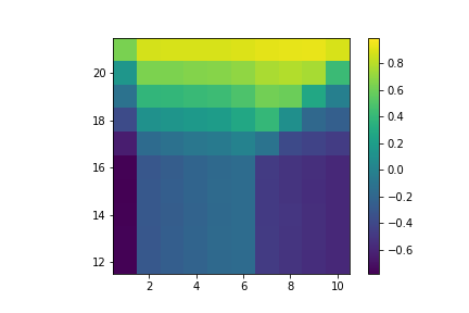
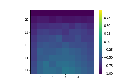
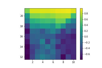
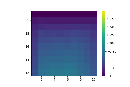
Here are the approximated State Value functions (x-axis is what card the dealer is showing and y-axis is the sum of our hand), we can see that the with an Ace is not as smooth as the one without since we encounter states without Ace much more often:

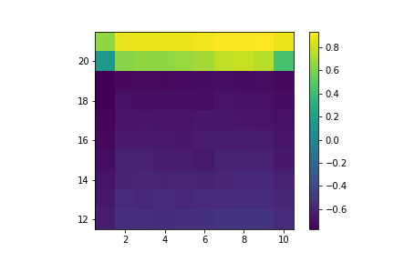
No Usable Ace

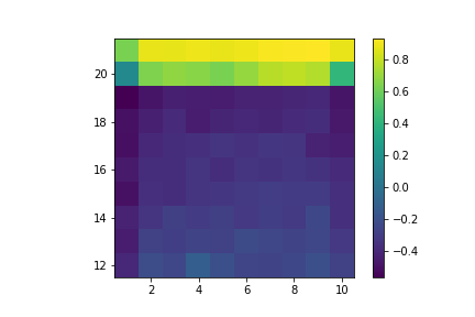
Usable Ace

Exploring Starts

If we do not have a model of the environment, we need approximations for state-action pairs, since creating a policy with state values requires the transition probabilities $p(s’, r \mid s,a)$. These actions values are also estimated by averaging sample discounted returns. The issue is that many state-action pairs might never be visited, and we need to estimate the value of all pairs to guarantee optimal convergence.

This is especially difficult if we have a deterministic policy, where only one action will be taken in each state. In other words, we need to ensure exploration of all actions for each state. One way is to only consider policies that are stochastic with nonzero probability for all state-action pairs. Another method is ‘exploring starts’, where every state-action pair has a non zero probability of being selected as the starting state of an episode.

Here’s the accompanying code:

usable = np.zeros((32, 11, 2, 2))
usable[1:22, 1:12] = 1

q = np.random.random((32, 11, 2, 2)) * usable
policy = np.argmax(q, axis=3)
ret = np.zeros((32, 11, 2, 2))
count = np.zeros((32, 11, 2, 2))

DISCOUNT = 1

for _ in range(10000000):
  # Environment already has positive chance for all states
  hand, show, ace = env.reset()
  state = (hand, show, int(ace))
  done = False
  episode = []

  action = np.random.randint(0, 2)
  (hand, show, ace), reward, done, _ = env.step(action)
  episode.append((state, action, reward))
  while not done:
    state = (hand, show, int(ace))
    action = int(policy[state])
    (hand, show, ace), reward, done, _ = env.step(action)
    episode.append((state, action, reward))
  
  g = 0
  while len(episode) > 0:
    state, action, reward = episode.pop()
    g = DISCOUNT * g + reward
    
    if (state, action, reward) not in episode:
      count[state + tuple([action])] += 1
      q[state + tuple([action])] += (g - q[state + tuple([action])])/count[state + tuple([action])]
      policy[state] = np.argmax(q[state])

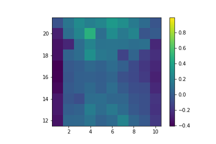
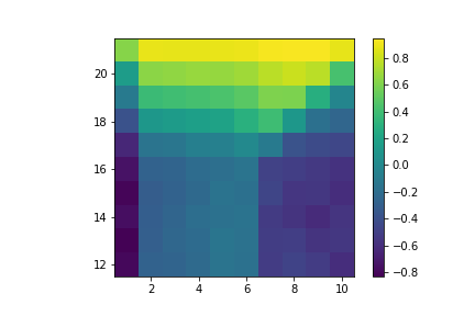
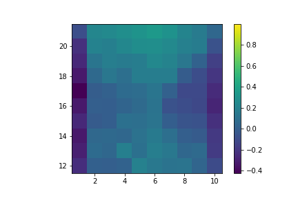
Which gives us:

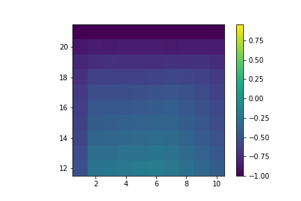
Value of hitting with no usable ace.

Value of hitting with a usable ace.

Value of sticking with no usable ace.

Value of sticking with no usable ace.

Policy Making

In Monte Carlo methods, we still want to follow the idea behind Generalized Policy Iteration, where we maintain approximate value and policy functions, and optimize them episode by episode. After each episode, the observed returns are used to update the visited states, and then the policy is improved for all these states.

There are 2 methods to go about approximating the optimal policy:

• On-policy means to evaluate or improve the policy used to generate the data.
• Off-policy methods evaluate or improve a different policy than the data generating one.

In on-policy, the policies are generally ‘soft’, as in the policy always has a non zero probability of selecting every action in every state, similar to the epsilon-greedy policies. We still use first visit MC methods to estimate action values.

Here is the code for on-policy control (learning the policy) on the Blackjack environment:

usable = np.zeros((32, 11, 2, 2))
usable[1:22, 1:12] = 1
q = np.random.random((32, 11, 2, 2)) * usable
policy = np.argmax(q, axis=3)
ret = np.zeros((32, 11, 2, 2))
count = np.zeros((32, 11, 2, 2))

epsilon = 0.1
DISCOUNT = 1

for _ in range(1000000):
  hand, show, ace = env.reset()  
  done = False
  g = 0
  episode = []

  while not done:
    state = (hand, show, int(ace))
    action = int(policy[state])
    (hand, show, ace), reward, done, _ = env.step(action)
    episode.append((state, action, reward))
  
  while len(episode) > 0:
    state, action, reward = episode.pop()
    g = DISCOUNT * g + reward
    
    if (state, action, reward) not in episode:
      count[state + tuple([action])] += 1
      q[state + tuple([action])] += (g - q[state + tuple([action])])/count[state + tuple([action])]
      g_action = np.argmax(q[state])

      if np.random.random() < epsilon:
        policy[state] = np.random.randint(0, 2)
      else:
        policy[state] = g_action

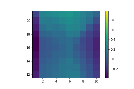
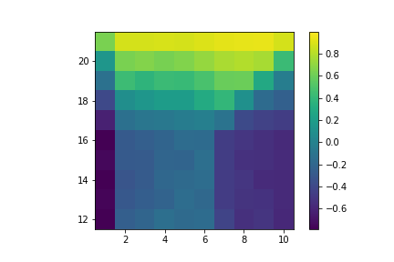
Here are the resulting value functions:

Value of hitting with no usable ace.

Value of hitting with usable ace.

Value of sticking with no usable ace.

Value of sticking with usable ace.

In off-policy, we consider 2 policies: a target policy $\pi$ that learns from the experience and becomes the optimal policy, and a behaviour policy $b$ which is more exploratory and generates the experience. Comparatively, on-policy is simpler and converges faster, but off-policy is more powerful and general (on-policy is a special case of off-policy when both target and behaviour policies are the same).

However, there is a problem when both $\pi$ and $b$ are fixed and we want to estimate $v_\pi$ or $q_\pi$. This is that the episodes follow $b$, while we try to estimate values for $\pi$, so we need to find a way to relate them to each other. To accomplish this, we require every action taken under $\pi$ also be taken in $b$, i.e. $\pi(a\mid s) > 0 \Rightarrow b(a\mid s) > 0$. This is also known as the assumption of coverage, it follows that $b$ must be stochastic where it is not identical to $\pi$, but $\pi$ can be a deterministic policy.

We approach this by utilizing Importance sampling, a technique for estimating expected values from one distribution given samples from another. This is applied to off-policy learning by weighting the sample returns according to the relative probability of their trajectories occurring under $\pi$ and $b$, called the importance-sampling ratio. The probability of the state-action trajectory $A_t, S_{t+1}, A_{t+1}, …, S_T$ occurring under $\pi$ is:

This still requires a model of the environment ($p(S_{t+1}\mid S_t, A_t)$), but if we consider the relative probability, we get:

So now we weight all our returns in $b$ with $\rho_{t:T-1}$ to transform it to returns for $\pi$. In doing so, let time continue to count up from episode to episode and we define:

• $\mathcal{T}(s)$: set of either all time steps when $s$ was visited (every visit method), or the first time steps of each episode when $s$ was visited (first visit method).
• $T(t)$: first episode termination after time $t$.
• $G_t$: return after time $t$ up until $T(t)$.

So we get:

• $\{G_t\}_{t \in \mathcal{T}(s)}$, the returns that matter to state $s$.
• $\{\rho_{t:T-1}\}_{t\in \mathcal{T}(s)}$, the corresponding importance-sampling ratios.

There are 2 ways of sampling each with their upsides and downsides:

• Ordinary importance sampling: \(V(s)=\frac{\sum_{t\in\mathcal{T}(s)}\rho_{t:T-1}G_t}{|\mathcal{T}(s)|}\)

• Weighted importance sampling: \(V(s)=\frac{\sum_{t\in\mathcal{T}(s)}\rho_{t:T-1}G_t}{\sum_{t\in\mathcal{T}(s)}\rho_{t:T-1}}\)

On one hand, Weighted importance sampling has a variance between ratios of at most 1, whereas Ordinary importance sampling has unbounded variance. On the other hand, the ordinary one is unbiased where the weighted one is. But with the assumption of bounded returns (which we can assume in most cases), the variance of Weighted importance sampling converges to 0, so in general Weighted importance sampling is better.

So our update for states with importance sampling weights $W_i$ and returns $G_i$ is:

Which can be constructed incrementally by keeping count $C_i$ and using:

b = np.ones((32, 11, 2, 2)) * 0.5
q = np.random.random((32, 11, 2, 2))
count = np.zeros((32, 11, 2, 2))
pi = np.argmax(q, axis=3)
DISCOUNT = 1

for _ in range(10000000):
  hand, show, ace = env.reset()
  done = False
  episode = []
  while not done:
    state = (hand, show, int(ace))
    action = np.random.choice(range(len(b[state])), p=b[state])
    (hand, show, ace), reward, done, _ = env.step(action)
    episode.append((state, action, reward))
  g = 0.0
  w = 1.0
  while len(episode) > 0:
    state, action, reward = episode.pop()
    sa = state + tuple([action])

    g = DISCOUNT * g + reward
    count[sa] += w
    q[sa] += (w * (g - q[sa])) / count[sa]
    pi[state] = np.argmax(q[state])
    if pi[state] != action:
      break
       
    w *= 1/b[sa]

Value of hitting with no usable ace.

Value of hitting with usable ace.

Value of sticking with no usable ace.

Value of sticking with usable ace.

For now that is all we need to know about Monte Carlo methods, but we will go much more in depth with Importance Sampling and its variants in the future.